What is Linear Regression?

In simplest terms, Linear Regression can be explained as just the curve fitting (straight line in this case) to the given set of data points. Linear Regression solves the following question: "Given a set of data points, what is the slope and y-intercept of the straight line which fits the data points perfectly?"

If you remember the elementry maths you would surely know the formula of a straight line, which is $y = mx + c$. Where, $m$ is the slope and $c$ is the y-intercept of the line!

Now when I say "the line which fits perfectly", that means the line placed in such a way that for any input $x$, it minimizes the difference between actual value (label: $y$) and the predected value $\bar{y}$. In our case, the predicted value is the point on the line at given $x$.

This cost function can be given by following equation and is called "Mean Squared Error" (Here I use $\theta_0$ and $\theta_1$ instead of $m$ and $c$ for slope and y-intercept respectively.) :

Where $y$ is actual value and $\bar{y}$ is predicted value.

If you wonder why we are using squared difference instead of absolute difference? Then this article is for you.

Our goal is to minimize the mean squared error (loss or cost). This can be iteratively done using Gradient descent. Here's the approach:

Intuition behind this equation is that gradient of curve at any point gives the direction of steepest ascent. But we are minimizing the error, So we need steepest descent and that's why there is `-ve` sign (Opposite of steepest ascent direction) in above equation.

Here, in above equation, $\theta$ is a vector with value:

Now, let's substitute the value of $\bar{y}$ in equation of MSE:

Now Let's implement this concept (We won't implement the vectorized version as explained above; as we will work with only 1 feature)

Let's first import required libraries:

import numpy as np # linear algebra
from sklearn.datasets import make_regression # For generating Linear regression dataset
from matplotlib import pyplot as plt

Now, for this tutorial purpose we won't use the actual dataset to train on, but instead we will generate the dataset on the fly as following:

X, y = make_regression(n_samples=100, n_features=1, noise=50, bias=10, random_state=666)

# reshape for the sake of simplicity
X = X.reshape(-1)
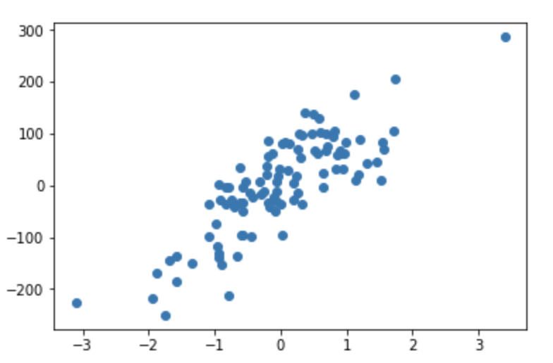
y = y.reshape(-1)

You can scatter plot the data generated by above function using following code:

plt.scatter(X, y)
plt.show()

Which should look similar to following plot:

Let's define some constants like learning rate $(\alpha)$

# CONSTANTS
LEARNING_RATE = 0.1 # alpha
TOLERANCE = 0.000001 # Convergence criteria
N = X.shape[0] # size of the dataset

Initially we don't know anything about $\theta_0$ and $\theta_1$. So we'll initialize both with 0 and start improving using gradient descent algorithm.

# Initialize weights with random number or 0.
theta0, theta1 = 0, 0

Let's create some helper function for calculating MSE and for making predictions.

def MSE(y, y_bar):
    return np.sum((y - y_bar) ** 2) / N

def predict(X, theta0, theta1):
    return theta0 + theta1 * X

Finally the gradient descent loop, in which I'll use the same equations explained above:

E_prev = 0
epochs = 0
while True:
    y_bar = predict(X, theta0, theta1)
    E = MSE(y, y_bar)
    theta0 = theta0 - LEARNING_RATE * ((-2/N) * sum(y - y_bar))
    theta1 = theta1 - LEARNING_RATE * ((-2/N) * sum(X * (y - y_bar)))
    if abs(E - E_prev) <= TOLERANCE:
        break
    E_prev = E
    epochs += 1
    print(f'MSE after {epochs} epochs: {E}')
print(f'Learned parameters: theta0 = {theta0} and theta1 = {theta1}')

The above training loop ends when the difference between consicutive errors is smaller than the $TOLERANCE$ defined in constants. It also prints the learned parameters.

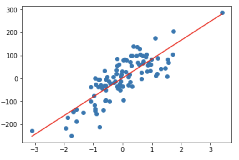
You can finally plot the dataset and the resultant best fit line using following code:

# Making predictions for plotting purpose
Y_pred = predict(X, theta0, theta1)

plt.scatter(X, y)
plt.plot([min(X), max(X)], [min(Y_pred), max(Y_pred)], color='red')  # plotting regression line
plt.show()

Which should look similar to following plot: